Stackelberg game §

1. 两家公司生产同一种产品的竞争，基本问题 §

ref: Stanford MS&E 246

• Firm 1和Firm 2生产同一种产品，产量分别为和，Stackelberg game假定Firm 1先行动，Firm 2后行动。

• Price per unit: 总产量越大，售价越低()

• Payoffs: 为第家公司的每件商品的成本，总收益即为生产件数乘以售价和成本的差

• 因为Firm 1先行动，所以在Firm 2确定产量时已知Firm 1的产量，那么应如何选择产量以获得最大收益：

  2. 二次函数求导可找出最值点 ，即为最大收益所对应的产量。 上式是在已知时的最佳应对策略。
  3. 令，即

• 由上式，Firm 1可以知道在自己决定产量后Firm 2将如何决策，那么在一开始决定最优产量时，有 和应根据以下两个条件进行讨论： Firm 1生产计划的目标是盈利，可得出边界条件。可推出，即 Firm 2应在保证自己不亏损的前提下规划生产（后订计划只能跟随Firm 1的制定好的策略），得到边界条件。可推出，即。 分两种情况讨论：

  1. ，即，Firm 2将进行生产 求导找出极值点 最优状态为： Firm 1的收益为： 实际情况中Firm 1的产品产量一定是正整数，即 这个条件和Firm 1一定会盈利等价，即同时满足。
  2. ，Firm 2将不会进行生产，则: 此时也应满足Firm 1生产盈利/产量不为负的条件。 化简后求导得，极值点应为。 判决与的关系
     1. 若，则，即，极值落在内，上单调递减，无法达到极大值，说明不应添加条件。 还是此时最优解应为celling()? 那么应有：，收益应大于0，必须满足，否则不应有。实际意义：若对方工厂成本更低，不可能通过提高产量迫使对方停产。
     2. 若（可得出），则，极值落在，满足约束，。 profit: 能否比较与

• 结论（需要再研究）

  的范围
  额外条件	None
  profit最优时
  profit		必须满足
  意义	需综合考虑最高售价、Firm 1和Firm 2的成本 决定产量->控制售价 当时的策略	此时售价接近于 即Firm 1以Firm 2的成本价销售让2无法盈利	额外条件告诉我们高于与中点 Firm1 以成本与最高售价中点定价实现最大利益

---

2. 攻防问题 §

2.1. Pure strategy §

Ref: Efficient algorithms to solve bayesian stackelberg games for security applications

Follower type 1	Follower type 2
C D A 2,1 4,0 B 1,0 3,2	C’ D’ A 1,1 2,0 B 0,1 3,2

• Leader’s strategies: . Follower’s strategies: . 当Leader选择strategy A，follower (type 1)选择strategy C时，leader的payoff为2，follower的payoff为1。Leader不知道Follower的payoff。 Follower type: can be different attackers taking place (e.g., leader move -> follower 1 move -> follower 2 move -> leader move -> …)

• Pure-strategy Nash equilibrium (player 1 and 2 select move at the same time, follower type 1):

  • The only Nash equilibrium for this game is when the leader plays a and follower type 1 plays c which gives the leader a payoff of 2.

  • A is strictly dominated:

    Note that, no matter how player 1 plays, R gives player 2 a strictly higher payoff than M does (2/6/8 vs. 1/4/6). In formal language, strategy M is strictly dominated. Thus, a “rational” player 2 should not play M. ---- Game theory, 1.1.2 Dominated strategies, p6

    • No matter how player 2 plays, A gives player 1 a strictly higher payoff than B does. So player 1 will choose A as its’ pure-strategy.
    • So Player 2 have to choose C.

• Pure-strategy, player 1 commit to an action first, then player 2 move:

  • Player 1 choose B and player 2 choose D.

• Example is adapted from Computing the optimal strategy to commit to. Use follower type 1. BD is (3, 1) in this paper.

  In this normal-form representation, the bottom strategy for the row player is strictly dominated by the top strategy. Nevertheless, if the row player has the ability to commit to a pure strategy before the column player chooses his strategy, the row player should commit to the bottom strategy: doing so will make the column player prefer to play the right strategy, leading to a utility of 3 for the row player. By contrast, if the row player were to commit to the top strategy, the column player would prefer to play the left strategy, leading to a utility of only 2 for the row player. If the row player is able to commit to a mixed strategy, then she can get an even greater (expected) utility: if the row player commits to placing probability p > 1/2 on the bottom strategy, then the column player will still prefer to play the right strategy, and the row player’s expected utility will be 3p + 4(1 − p)=4 − p ≥ 3. If the row player plays each strategy with probability exactly 1/2, the column player is indifferent between the strategies. In such cases, we will assume that the column player will choose the strategy that maximizes the row player’s utility (in this case, the right strategy). Hence, the optimal mixed strategy to commit to for the row player is p = 1/2.

• Learning and approximating the optimal strategy to commit to Use follower type 1. BD is (3, 1) in this paper. Rows are U and D, coloumns are L and R.

  For the case where the players move simultaneously (no ability to commit), the unique Nash equilibrium is (U, L): U strictly dominates D, so that the game is solvable by iterated strict dominance. So, player 1 (the row player) receives utility 2. However, now suppose that player 1 has the ability to commit. Then, she is better off committing to play D, which will incentivize player 2 to play R, resulting in a utility of 3 for player 1. The situation gets even better for player 1 if she can commit to a mixed strategy: in this case, she can commit to the mixed strategy (.5 − , .5 + ), which still incentivizes player 2 to play R, but now player 1 receives an expected utility of 3.5 − .

2.2. Bayesian Stackelberg games §

2.2.1. case 1: §

• Method to solve a Bayesian Stackelberg game:
  • Use Harsanyi transformation, then Multiple-LPs (optimal strategies) or MIP-Nash (Nash equilibrium)
  • Assume type 1 will be active with probability , and type 2 will be active with probability

	CC’	CD’	DC’	DD’
A	, 1	,	,	,
B	,	,	,	,

2.2.2. case 2: §

Ref: Playing repeated Stackelberg Games with unknown opponents

	Leader agent	follower agent
	Single type 只有一组策略（如上表中type 1）	type drawn from a set 有多组策略（如同时存在上表中type 1和type 2）
set of pure strategies
utility function		Unique for each type
Select action	First commiting to a mixed strategy is the probability of the leader executing	By given and select type , best response pure strategy, satisfies
expected utility	If know , then

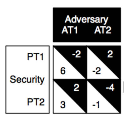
（不太确定PT2，AT2的leader payoff是不是错了？应该是+1？和后面的图以及2.2的推导不一致）

	Leader	Follower
策略	pure strategy为 : patrol T1 : patrol T2	pure strategy为 : attack T1 : attack T2
utility function	表格中对应的Leader的收益（白色）	表格中对应的Follower的收益（黑色） 每种对应收益唯一，即此问题中只有一个元素
	不妨假设，， 则会有一半的几率patrol T1，另一半几率patrol T2	对Follower为已知 AT1的期望收益为 AT2的期望收益为 那么，attack T1

若Leader patrol T1，follower attach T1，则leader收益为6，follower收益为-2。 Leader的策略为：有的概率去patrol T1，的概率patrol T2。此时若follower选择attack T1，预期收益为；若attack T2，预期收益为。 所以为follower选择的分界点，时follower将attack T1，时将attack T2，时follower无论选择哪个terminal都会获得同样的收益(“assuming that the follower breaks ties in the leader’s favor”，follower选T1对leader有利)。

• 时，leader预期收益为，单调增。
• 时，leader预期收益为，单调减。 所以为最佳策略，follower将优先选择attack T1，那么leader预期收益为。

2.3. Repeated game formulation (接case 2) §

此处PT2, AT2时Leader的payoff设置为1，而不是图中的-1

• po: payoff for the leader
• u11, u12, u21, u22分别为(PT1, AT1), (PT1, AT2), (PT2, AT1), (PT2, AT2)处follower的payoff，未知
• EU: expect utility.

---

3. TODO: 古诺双寡头 §